Darboux integration

Darboux integration (or Riemann integration) is similar to what we learned in Calc. In Analysis, we broke down how the integral sign is composed of these series (Darboux sums), which goes back to the idea of approximating the area under a curve with a bunch of rectangles.

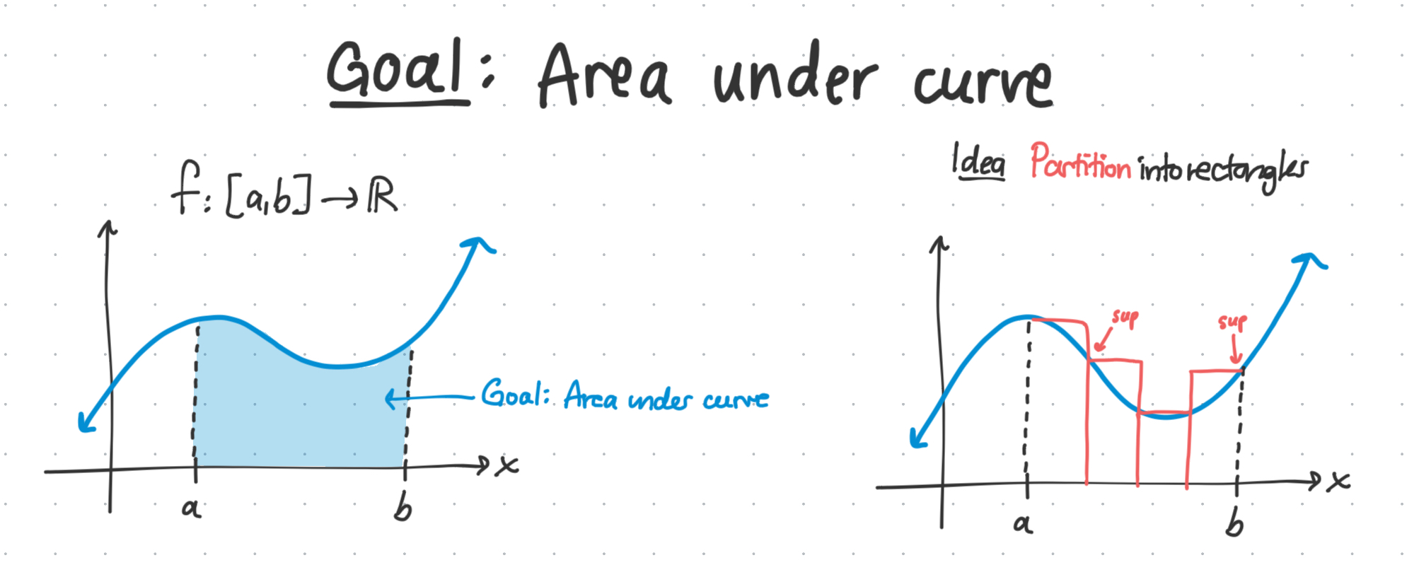
In calculus, we learned that we can construct a Riemann approximation using left, right, midpoint, and trapezoidal approximations. These were really only specific, easy-to-understand examples of Darboux sums computed over certain partitions.

Darboux integration: The setup

The partition

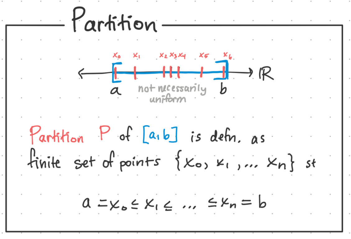
The partition $P$ is basically any finite set of points which splits up (‘partitions’) an existing interval into subintervals. This is the base for which we’re going to define rectangles on top of.

Darboux sums

Now, let’s take any given partition and try to form one estimate for the area under our curve.

The Darboux sum has two variants - the upper and lower Darboux sums.

The upper Darboux sum is the largest possible area we can get by summing over the rectangles formed by given partition. We define it as the following:

\(U(P, f) = \sum^n_{i=1} \sup_{x \in \Delta x_i} f(x) \Delta x_i\) Where $\Delta x_i$ is just the width (the change in x) of the given $i^{th}$ subinterval within the partition.

The lower Darboux sum is the smallest possible area we can get by summing over the rectangles formed by given partition. We define it as the following:

\(L(P, f) = \sum^n_{i=1} \inf_{x \in \Delta x_i} f(x) \Delta x_i\) Where the only difference from the upper variant is that we take the $\inf$ over all $x$ in the subinterval as the $f(x)$ point. And again, this is only for ONE given partition.

Darboux integral

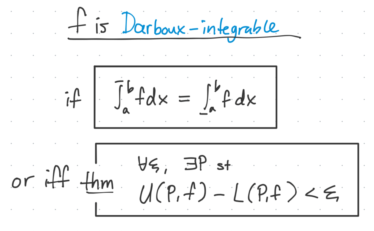
The Darboux integral is special in that it goes through ALL POSSIBLE partitions of the interval and it finds the one either minimizing the area of $U(P, f)$ or maximizing the area of $L(P, f)$. As such, it comes in two variants as well.

The intuition is that if these two upper and lower integrals are equal or epsilon-close to each other, then we consider the function $f$ to be Darboux-integrable. Hooray!

Integral properties

Linearity of integration

• Addition
• Scalar multiplication Integral comparisons Splitting integrals Bounded by area of rectangle

What is integrable?

The following types of functions are integrable.

Continuous functions

The following result is a very important property of continuous functions - that all continuous functions in $\mathbb{R}$ are Darboux integrable.

How do we prove this? We use the idea that if $f$ is continuous in a compact space ($[a,b]$ is compact in $\mathbb{R}$), it implies $f$ is also uniformly continuous.

Monotone increasing + bounded functions

If $f:[a,b]\rightarrow \mathbb{R}$ is bounded and monotone increasing (or decreasing), then $f$ is Darboux integrable.

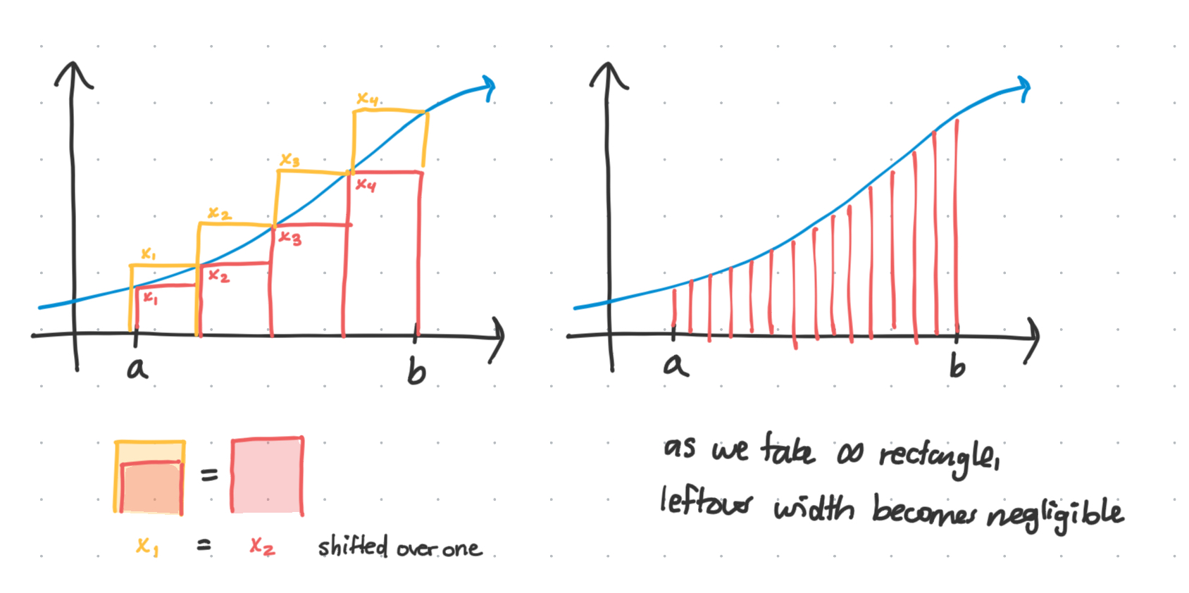
Proof sketch: Create an equidistant partition where each $\Delta x_i$ is super small. Then create the upper and lower Darboux sums and try to make them epsilon close by shifting the indices of the sum.

Special compositions

$g[f(x)]$ is integrable when $f$ is bounded and integrable, and $g$ is continuous.

Fundamental theorems of calculus

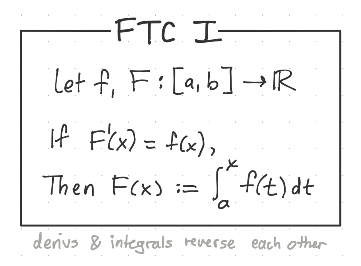
FTC I: Defining the inverse relationship

The first fundamental theorem of calculus is essentially saying that the definite integral reverses differentiation.

FTC II: Helping us compute it

The second fundamental theorem of calculus allows us to compute the definite integral as the difference between the antiderivatives at $F(b) - F(a)$.

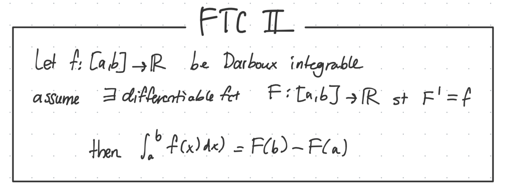
The proof stems from creation a partition and using MVT to show that there exists some point which looks like the \(F(x_j) - F(x_{j-1}) \quad j=1, 2, 3, \cdots n\) across all $n$ partitions. Then using that we can finesse the integral equation into looking like $F(b) - F(a)$.

Integration techniques

Integration by parts

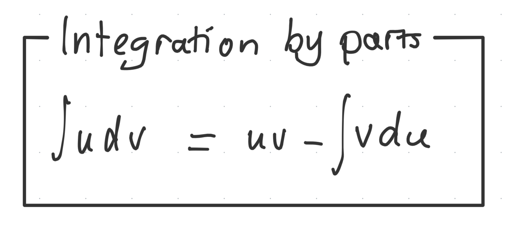
The proof stems from applying the product rule, FTC, then rearranging to get our desired result.

Change of variables

Finally a useful trick to know when working with integrals is how to change the variable of integration.

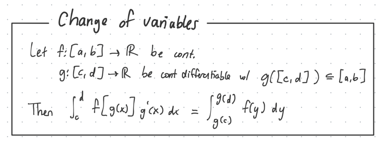
In practice, it works by identifying terms which look like the inverse of a chain rule operation. Then simplifying it into the outer function only, and then changing the bounds of integration and the variable of integration by solving their respective equations.