Derivatives

Finally - differentiation!!

Using our epsilon-delta definition of limits / continuity, we finally have the tools to unpack rigorously the iconic limit definition of differentiation. This blog post will break down how we define the derivative, the different rules + ideas for how to prove them, and talk the Rolles -> MVT -> generalized MVT pipeline.

The derivative

The derivative describes the instantaneous slope / rate of change of the function at the given time.

Precisely, it has the definition of taking a small change in x, passing the difference through the function, then dividing it by the change in x to get the ‘rise’ over ‘run’ of the function at the given point. And we take the limit as the run gets infinitely small to find very precisely what is the slope at this point.

Every differentiable function is continuous

Recall that the definition of continuity looks like having the limit of $f$ as $h$ approaches some small neighborhood around $x$, look like $f(x)$. \(\lim_{h\rightarrow 0}f(x+h) = f(x)\) Doesn’t this look kind of similar to our derivative definition? We can easily rearrange.

Derivative rules

The proof of all these rules follows from regurgitating the derivative definition given above, and doing a bunch of algebra.

Sum rule

The sum rule follows from the linearity of differentiation, which is to say that:

\((f+g)^\prime (x) = f^\prime(x) + g^\prime(x)\) The proof takes 3 lines.

Product rule

The product rule is one I had drilled into me from my high school Calculus class.

\((fg)^\prime(x) = f^\prime(x)g(x) + f(x)g^\prime(x)\) The proof of this requires more massaging, and the addition / subtraction of a $f(x+h)g(x)$ term in the numerator. A tip for the proofs is to think about the final format which we want to get the equations in. So if we know the end goal is to get a $f’(x)g(x)$ term, then we would want to use the derivative definitions and see what algebraic manipulations can be done to get the equation into that form.

Power rule

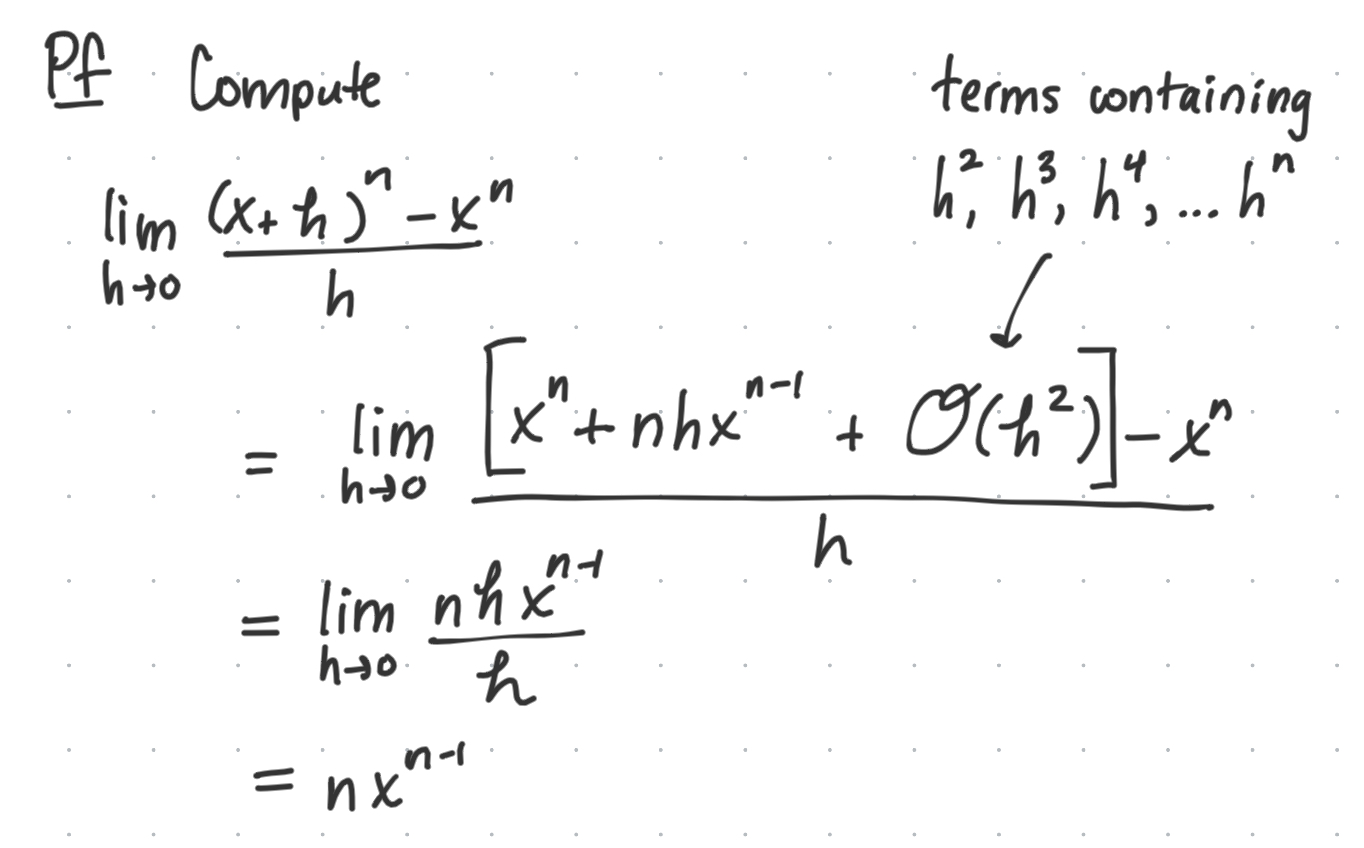
The power rule is one that we start to feel intuitively and abstractly, through many pages of introductory derivative practice.

\[\begin{align*} f(x)&=x^n\\ \implies f^\prime(x)&=nx^{n-1} \end{align*}\]

The proof of this requires a weird $O(h^2)$ term, which goes to zero since we take the $\lim_{h\rightarrow 0}$.

Chain rule

The chain rule acts on two differentiable functions and says, if you have two differentiable functions $f, g$ and take the composition $g \circ f$ or $g[f(x)]$, then take the derivative of this new composed function, then it is equivalent to taking the derivative of the outside function, multiplied (or ‘chained’) on with the derivative of the inside function.

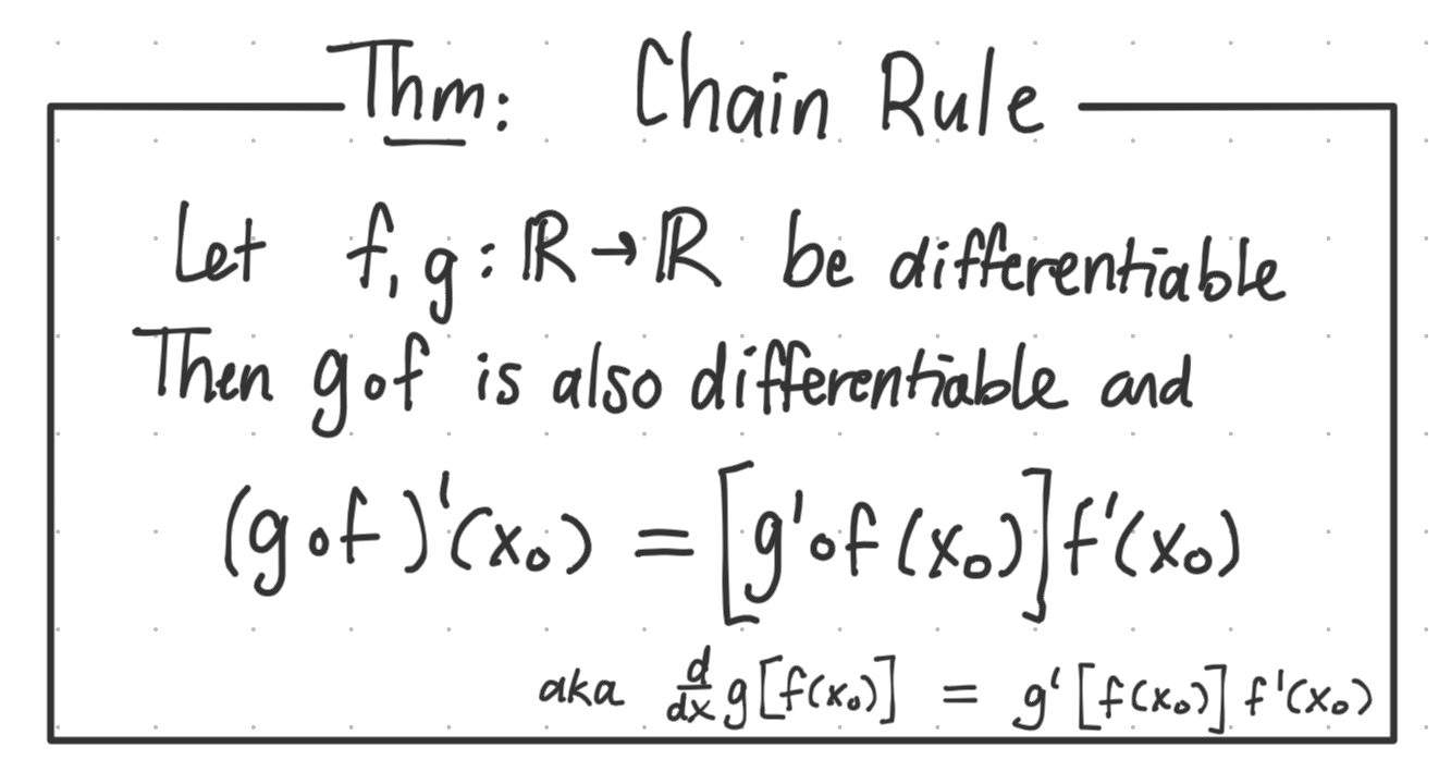
Note that this can occur for multiple chains, and multiple (more than just 2) layers of nested compositions.

The proof of the chain rule is the most complicated of these four rules. I’m going to black box it for right now since my final is in two hours and I have two other sections (Integration and Sequences of Functions) to get through.

MVT

Local maxima

$x_0$ is a local maximum of $f$ if there exists a $\delta$-neighborhood which $f(x)$ for all $x$ within this radius of $x_0$ satisfy $f(x_0) \geq f(x)$

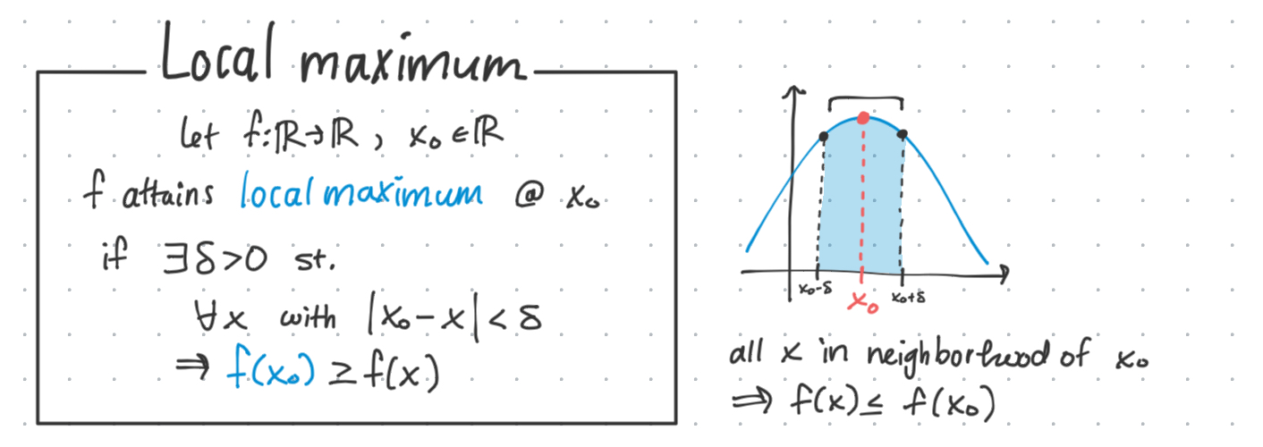
Prop: We can say the derivative $f^\prime(x_0)=0$ at local maxima. This can be observed graphically and proved with derivative definition regurgitation.

Rolle’s theorem

Rolle’s theorem states that if you have a differentiable function $f:[a,b]\rightarrow \mathbb{R}$ defined on some interval $[a, b]$ such that $f(a) = f(b)$, we know that there must be SOME point $x_0$ within $[a,b]$ such that $f^\prime(x_0)=0$.

We can observe this graphically just by trying to draw a continuous line (since differentiable $\implies$ continuity) between two points with the same $y$-value without creating a horizontal tangent line.

I wish there was a nice way to remember this, but honestly it’s best thought of as being able to ‘roll’ something along a horizontal tangent line if the boundaries are the same height. Sucks it couldn’t have a more descriptive name, but I suppose Rolle had to be narcissistic.

Mean value theorem

The mean value theorem is like an overpowered version of Rolle’s theorem, in that it guarantees we can find a point (a ‘value’) within $[a,b]$ that has the derivative equivalent to the ‘mean’ of the rise/run across the entire interval. Which is difficult to put into words exactly and I think is much more easily explained with a picture.

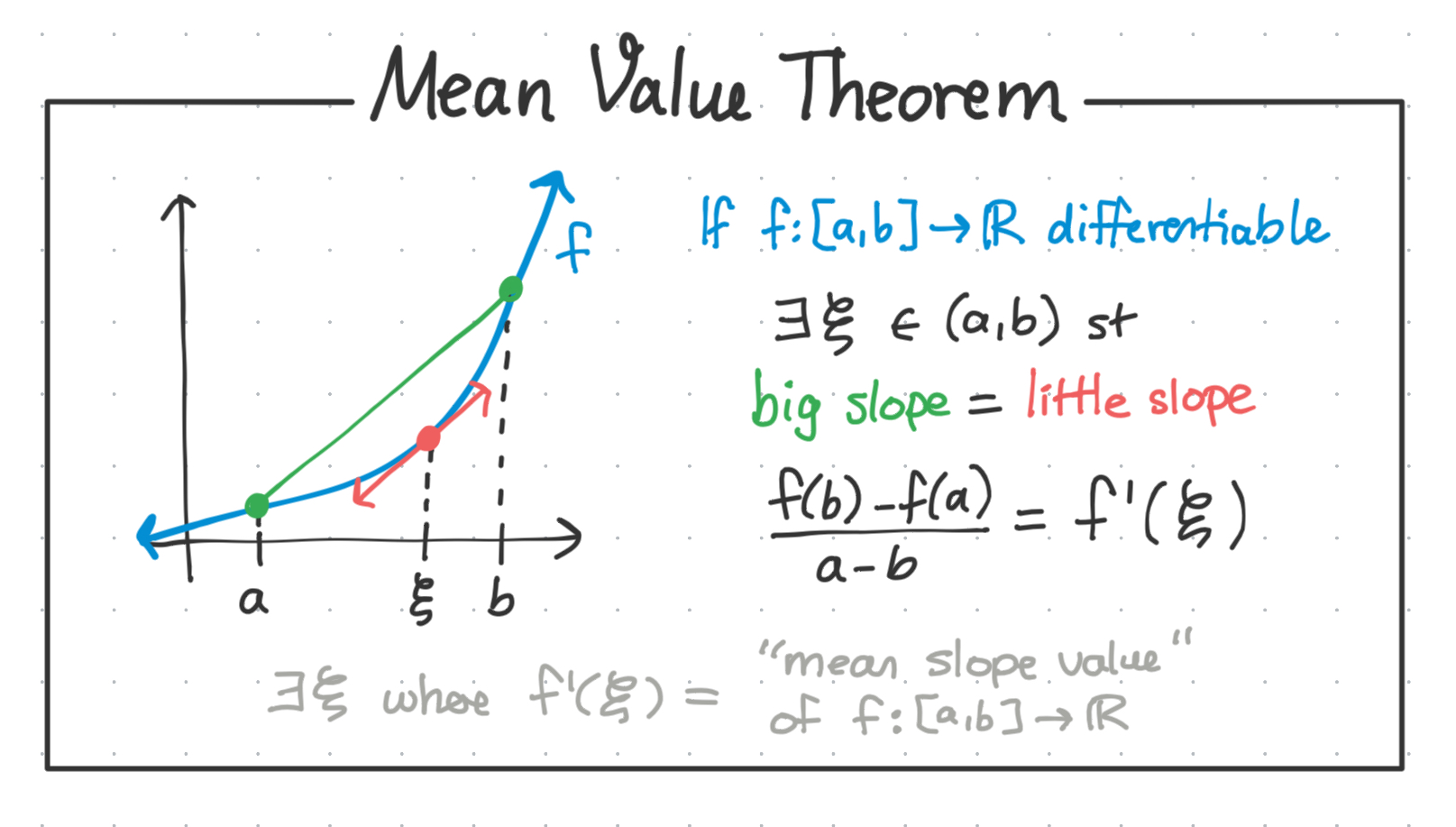
A similar sanity check can be done by trying to draw a continuous line between two points of differing heights and avoiding drawing some line which creates a tangent with the same slope as the bigger slope.

And indeed, plugging in $f(b) = f(a)$ into the mean value theorem gets us the same result as Rolle’s theorem. Fuck you Rolle.

Generalized MVT

The generalized MVT is the final evolution in the Rolle $\rightarrow$ MVT pipeline. It states that there is some point (‘value’ again) within $[a,b]$ such that the ratio between the derivatives of $f$ and $g$ at that point is equivalent to the greater ratio of the ‘mean’ rise/runs of $f$ and $g$.

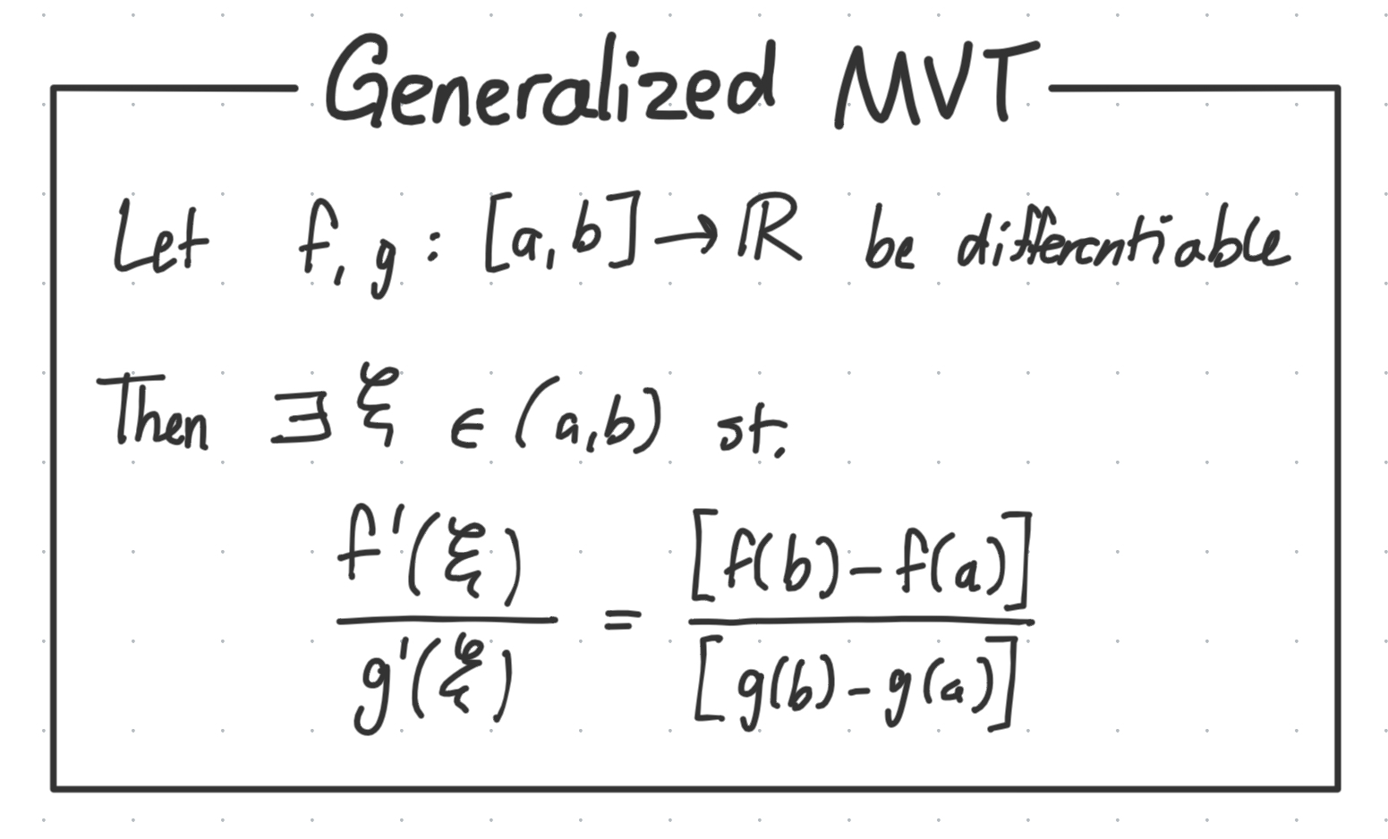
The normal MVT is just the generalized MVT but taking $g(x) = x$. 🤯

L’hopital’s rule

L’hopital’s rule lets us find the value of $\lim_{x\rightarrow a}\frac{f(x)}{g(x)}$ when both $f$ and $g$ go to $0$ in the normal world, but don’t in the (nth) derivative world.

It basically says it suffices to find: \(\lim_{x\rightarrow a}\frac{f^\prime(x)}{g^\prime(x)} = \lim_{x\rightarrow a}\frac{f(x)}{g(x)}\)

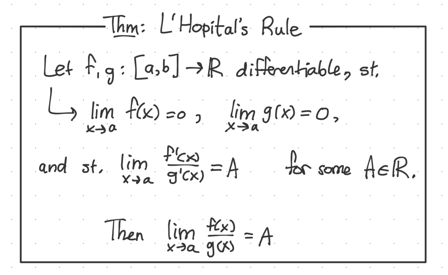
There is also no memory aid for tying the name to the function. We just have to remember that L’hopital helps us with limits going to 0/0.