Training a neural network to poorly predict sailboat prices…

Tonight, I wanted to finally teach myself how to use PyTorch (mostly so I can say I’ve used PyTorch before in my interview tomorrow). I already went through the work of scraping and preprocessing some sailboat economic data for the Columbia Mathematical Modeling Workshop, so I thought it would be a good launching point to run through the torch machine.

I first imported the necessary libraries:

import torch
import torch.nn as nn
import torch.optim as optim
import pandas as pd
import matplotlib.pyplot as plt
from sklearn.model_selection import train_test_split
from sklearn.preprocessing import StandardScaler

Here we read in the data and perform some simple data visualization to inspect what it looks like.

# Read in catamaran sailboat data (pre-processed in R)
cat_data = pd.read_csv('data/cat_data.csv')

# Tensorize numeric columns
X = cat_data[['length', 'price', 'year', 'gdp', 'hdi']]
Y = cat_data['price'] # Target variable
X = torch.tensor(X.values, dtype=torch.float32)
Y = torch.tensor(Y.values, dtype=torch.float32)

# Split data into train and test sets
X_train, X_test, Y_train, Y_test = train_test_split(X, Y, test_size=0.2, random_state=42)

# Normalize data
scaler = StandardScaler()
X_train = scaler.fit_transform(X_train)
X_test = scaler.transform(X_test)

# Visualize the training data
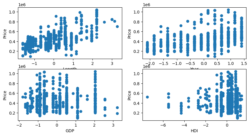
figs, axs = plt.subplots(2, 2, figsize=(10, 5))

# Plot length vs price
axs[0, 0].scatter(X_train[:, 0], Y_train)
axs[0, 0].set_xlabel('Length')
axs[0, 0].set_ylabel('Price')

# Plot year vs price
axs[0, 1].scatter(X_train[:, 2], Y_train)
axs[0, 1].set_xlabel('Year')
axs[0, 1].set_ylabel('Price')

# Plot gdp vs price
axs[1, 0].scatter(X_train[:, 3], Y_train)
axs[1, 0].set_xlabel('GDP')
axs[1, 0].set_ylabel('Price')

# Plot hdi vs price
axs[1, 1].scatter(X_train[:, 4], Y_train)
axs[1, 1].set_xlabel('HDI')
axs[1, 1].set_ylabel('Price')

plt.show()

Interestingly, it seems the most correlated variable in determining a sailboat’s price is its beam length. GDP and HDI seem to have very little correlation.

Next, we create a simple neural network with 3 layers.

1. The input layer, defined by the 4 independent variables in our sailboat dataset.
2. self.fc1 and self.fc2 are two hidden layers. The first has 64 nodes, the second has 34.
3. Finally, the ouput layer has 1 final node, representing the price of the sailboat.

class SimpleNN(nn.Module):
    def __init__(self, input_size):
        super(SimpleNN, self).__init__()
        self.fc1 = nn.Linear(input_size, 64)
        self.fc2 = nn.Linear(64, 32)
        self.fc3 = nn.Linear(32, 1)

    def forward(self, x):
        x = torch.relu(self.fc1(x))
        x = torch.relu(self.fc2(x))
        x = self.fc3(x)
        return x

Putting it all together, we initialize our model, the loss and optimizer functions, and train it over 100 epochs (iterations).

# Initialize the model
input_size = X_train.shape[1]
cat_model = SimpleNN(input_size)

# Loss function and optimizer
criterion = nn.MSELoss()
optimizer = optim.Adam(cat_model.parameters(), lr=0.01)

# Train the model
num_epochs = 100
for epoch in range(num_epochs):
    cat_model.train()
    optimizer.zero_grad()
    outputs = cat_model(torch.tensor(X_train, dtype=torch.float32))
    loss = criterion(outputs.squeeze(), Y_train.clone().detach())
    loss.backward()
    optimizer.step()
    if (epoch+1) % 10 == 0:
        print(f'Epoch [{epoch+1}/{num_epochs}], Loss: {loss.item():.4f}')

# Evaluate the model... (it doesn't perform very well yet)
cat_model.eval()
with torch.no_grad():
    outputs = cat_model(torch.tensor(X_test, dtype=torch.float32))
    loss = criterion(outputs.squeeze(), Y_test.clone().detach())
    print(f'Loss: {loss.item():.4f}')

Epoch [10/100], Loss: 225700364288.0000
Epoch [20/100], Loss: 225678917632.0000
Epoch [30/100], Loss: 225616642048.0000
Epoch [40/100], Loss: 225472921600.0000
Epoch [50/100], Loss: 225189330944.0000
Epoch [60/100], Loss: 224690487296.0000
Epoch [70/100], Loss: 223887572992.0000
Epoch [80/100], Loss: 222681792512.0000
Epoch [90/100], Loss: 220966977536.0000
Epoch [100/100], Loss: 218633568256.0000
Loss: 222609850368.0000

A loss of 222609850368.0000….. not great. I don’t have time to investigate further for tonight (I have to write a reading response to the Communist Manifesto by tomorrow), but I feel accomplished having actually trained my first model from scratch!

I’ll report back later to see if I can’t improve upon these results.