How MOSES paints with symmetries

Gang lab: Self assembling materials

The Gang lab is a materials science lab focused on the fascinating problem of self assembling materials.

Our fundamental building block is the DNA origami - octahedral wireframes (voxels), loaded with nanoparticle cargo, which self assemble via the unique strands of DNA connecting them together (bonds). Millions of these babies come together in an annealing machine, enabling us to form these organized, customizable crystal structures.

My role has been to work on the formalization + continuation of MOSES (Mapping Of Structurally Encoded aSsemblies): An algorithm for deducing a coloring scheme for these bonds which reduces the number of unique origami while still retaining the essential particle structure of the lattice.

We bookended this project this semester, culminating in our paper being published to ACS nano and even being featured on the front cover!

Now, my project is extend the MOSES algorithm to more complicated / non-octahedral designs. To that end, I wanted to boil down the essential guts of the current algorithm — so in this blog post, I want to continue from where I left off last time; explaining the intuition behind the algorithm behind how exactly MOSES designs these DNA origami building blocks.

Our self assembly problem

Lattice: The pattern

Stepping back into 2D again, imagine you wanted to assemble the following beautiful lattice pattern:

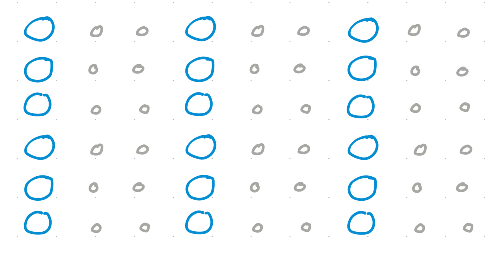
Which tiles out like this for infinity.

Voxels: The building blocks

But, this pattern needs to self assemble. Moreover, all we have control over is the design of each voxel - namely, in the specificity (abstracted as ‘color’) of the bonds attached to a given voxel in the $\pm x, \pm y$ directions.

• Recall: green+ only binds with green-, red+ only binds with red-, etc.
• Let’s define an origami to be the combination of both a voxel + its four bonds

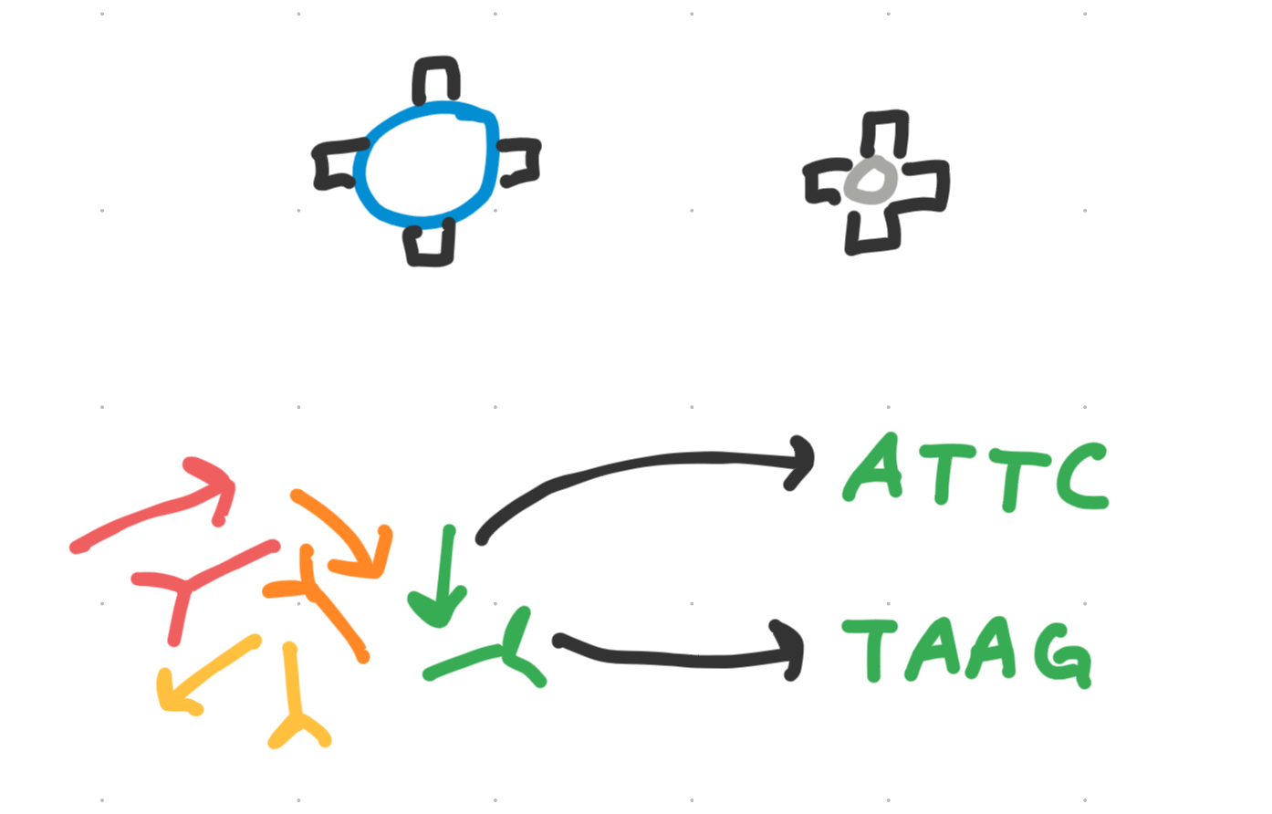
So, how would we ‘color’ the vertices of each voxel in the lattice so that we create our desired pattern?

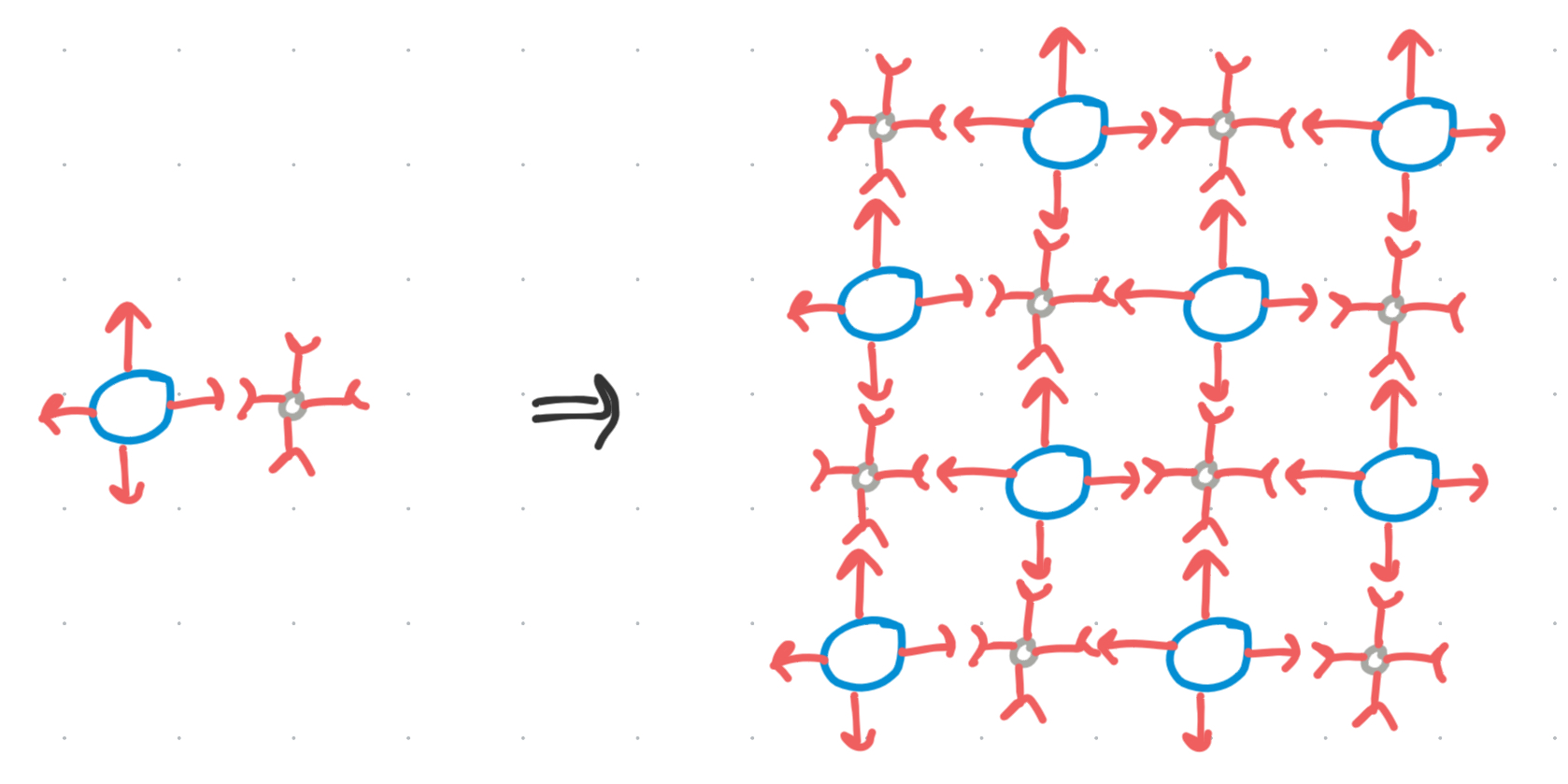
A bad coloring job

For example, this coloring from my previous post would NOT give us the structure we wanted.

The MOSES algorithm

The idea

The idea underpinning the MOSES algorithm is to reduce the number of colors based on the symmetries between different voxels in the lattice.

Where two voxels $v_{1}, v_{2}$ are defined to be ‘symmetric’ if there exists a rotation which can transform their surroundings so that they look the same

The problem: revisited

The lattice setup

We can model the symmetries of our lattice as a group $G$ acting on a set, our lattice $\mathcal{S}$.

Where the group $G$ is the set of rotations which take the $\mathbb{Z}^2$ lattice to itself (which are the same as the group of rotations on a square):

\[G = \{0 ^{\circ}, 90 ^{\circ}, 180 ^{\circ}, 270 ^{\circ}\}\]

And the set is the infinite tiling lattice:

\[\mathcal{S}= \left\{ (x, y) | x,y \in \mathbb{Z} \right\}\]

And returning to our goal pattern:

We can model the different particle locations as a function $C:\mathcal{S}\to \mathbb{N}$ atop the lattice which maps points to ‘colors’, where $1$ is the blue particle, $0$ is the empty. Say we choose the following function.

\[C(x, y)= \begin{cases} 1, \quad x \% 3 = 0 \\ 0, \quad \text{else} \end{cases}\]

The minimum design

To simplify things, lets reduce this to a smaller subset which could be copy-pasted infinitely to form our desired structure. Let’s call it our minimum design.

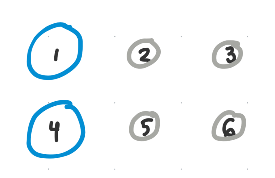
Now, since all we care about is designing a unique set of voxels — within here, what voxels can we reuse?

Symmetry through voxel surroundings

Revisting the idea of symmetry, we deviate a little from the standard definition of lattice symmetry and consider the point symmetry of any given point (voxel) in $\mathcal{S}$ compared to the other voxels.

The idea is, that if the lattice looks the same around some $v_{i}$ as it does around $v_{j}$, then we can say $v_{i} \equiv v_{j}$.

Reducing the $O(\infty)$ endeavor

However, making all comparisons of a $\mathbb{Z}^2$ lattice would take infinite time. But it suffices to take each voxel in this design as the center of its own ‘unit cell’, encapsulating all the information of the global lattice. Calling these the ‘voxel surroundings’, we can enumerate the different symmetries of each voxel with respect to each other without having to compute the transformations on the entire lattice.

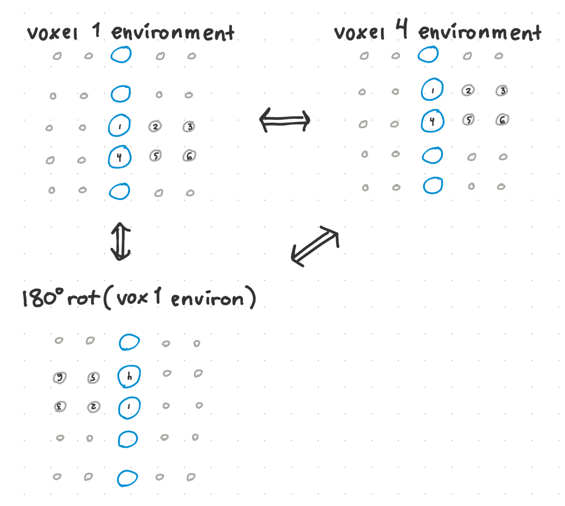
Since we know what the environment of each voxel should be, we compute the symmetry between $v_{1}, v_{2}$ via the following method:

1. Tile out the surroundings centered around $v_{1}$
2. Rotate $v_{1}$’s surroundings with the rotation $r$ to check
3. Overlay $v_{1}$ surroundings on top of $v_{2}$’s surroundings and see if they are the same

If two voxels have some symmetry $r$ between them, then what this means for self assembly is that if $v_{1}$ rotates via $r$, then it would also be able to safely slot into $v_{2}$’s position in the lattice.

Example: Symmetry($v_{1}, v_{4}$)

For example, $v_{1}$ and $v_{4}$ in our design have $180 ^{\circ}$ symmetry, as illustrated by the following:

Formalizing voxel symmetry: Groups, actions, and orbits

Formally, we can define a function $F:\mathcal{S}\to\mathcal{S}$ taking the voxel’s coordinates in the original infinite lattice to its voxel surroundings. It would translate the voxel $\vec{x}$ to be in the center of a new square of its surroundings, big enough to encapsulate all the information of the original lattice under all rotations:

\[\begin{align} F(\vec{x}) = \{ (x,y) \in \mathcal{S} | x \in [-m, m], y \in [-m, m] \} \end{align}\]

Where $m$ is the maximum length of the minimum design - in our case, $3$.

Moreover, we can compare the colorings of $F$ by defining following action:

\[G \circlearrowright F(\mathcal{S}), \quad \text{with }g \cdot F(s) = F(g^{-1} \cdot s)\]

This way, we can define the symmetry groups of specific voxels within the lattice via the orbits of this action, where voxels are all prescribed to certain equivalence classes based on whether they can transform into each other with some rotation.

For our example, we get the following equivalence classes:

\[\begin{align} [v_{1}] &= \{ v_{1}, v_{4} \} \\ [v_{2}] &= \{ v_{2}, v_{3}, v_{5}, v_{6} \} \end{align}\]

Awesome, so how does this inform our final coloring?

Coloring with equivalences

We have the notion that voxels in $[v_{1}]$ can look the same, and voxels in $[v_{2}]$ can look the same, so long as they are rotated with respect to the transformation which put them in the equivalence class in the first place.

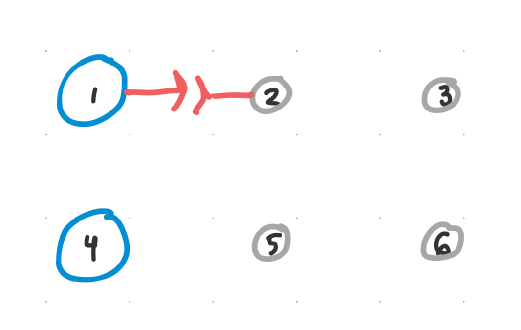
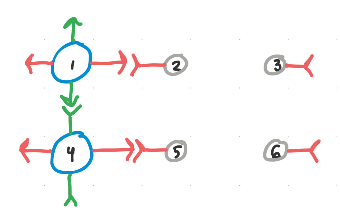
Our first color

We know for sure that $v_{1}$ and $v_{2}$ have to be different, and that there should be a unique color connecting those two. So let’s paint a red bond connecting $v_{1}$ and $v_{2}$. Again note that $r+$ and $r-$ are different, but complementary strands of DNA.

Now, we know that $v_{1}$ has a $180 ^{\circ}$ self-symmetry with itself. Likewise, it has translational and $180 ^{\circ}$ symmetry with $v_{4}$. So we map those colors onto the rest of the equivalence class, with the understanding that we could technically swap out the locations of any , rotate it with its symmetry, and the surrounding lattice will remain unaffected.

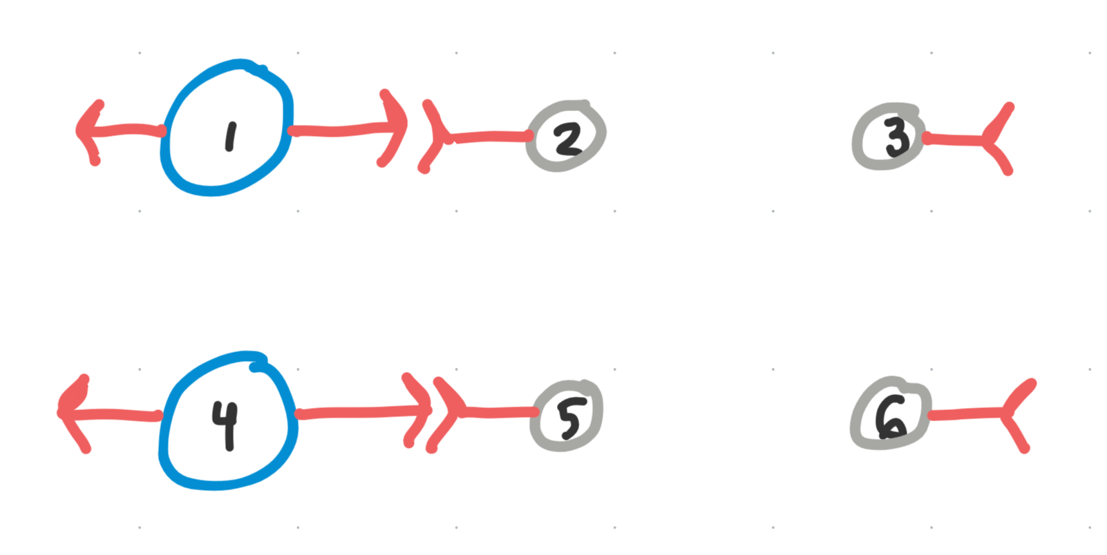
And if they are painted that color, their partner must have the color of the opposite complementarity on its connecting vertex. so we paint those too.

We end up with a partially-colored lattice.

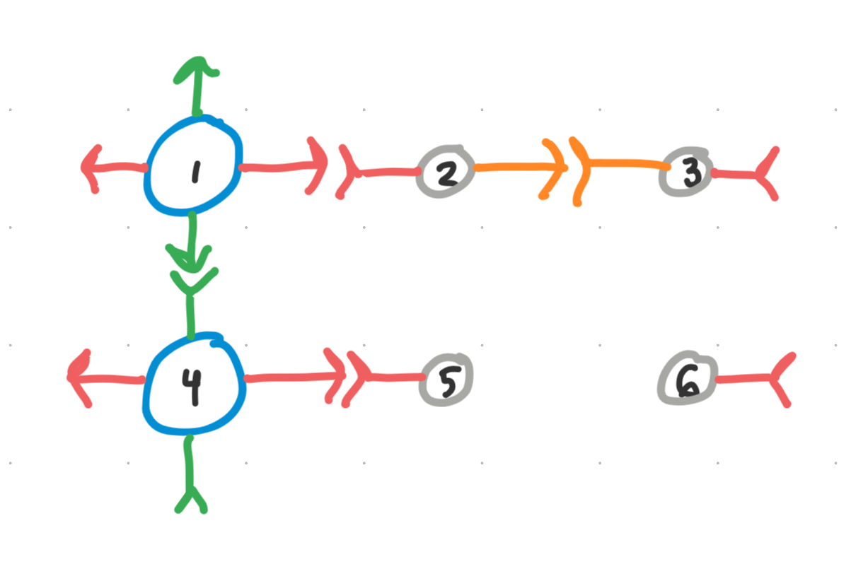
Our second color: A ‘complementary’ bond

in some cases, this structural painting + equivalence class mapping is enough to paint the entire lattice. But in our example, we are not done painting.

We have to add in another color because if we reused red, we would end up with the scenario illustrated in the “A bad coloring job” section.

So we need to add in another color, say green, connecting $v_{1}$ and $v_{4}$ together.

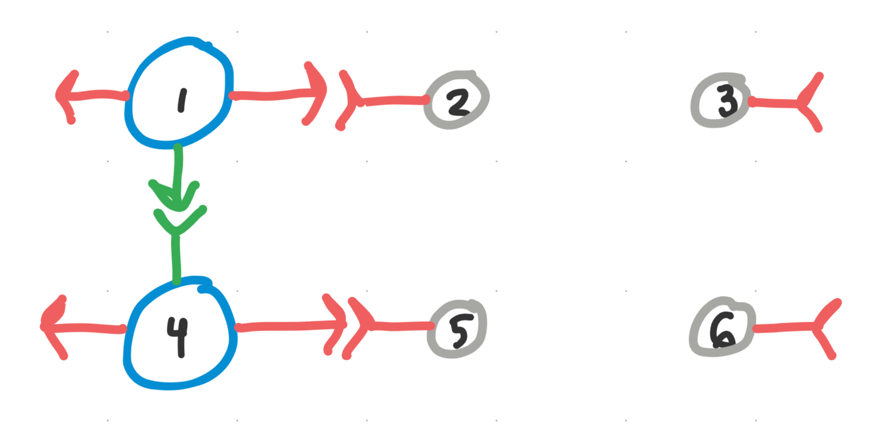
But now, $v_{1}$ and $v_{4}$ are no longer interchangeable in the system - they are completely different building blocks.

Again, we try to use the self-symmetries to reuse this green color as much as we can. However, one of the binding rules determined by our experimentalists was that we cannot allow for “palindromes”, where we have a color and its complement on the same voxel.

Hence, we cannot just apply the same kind of translational mapping that we did with the red bond. Instead, we map the voxel to itself with its $180 ^{\circ}$ self symmetry as such.

Now we have 3 distinct voxel types, in the wake of having broken $[v_{1}]$ into two new sub-classes, forced into existence by the double sided nature of DNA.

\[\begin{align} [v_{1}] &= \{ v_{1}, v_{4} \} \\ \implies [v_{1}]^+ = &\{ v_{1} \}, \quad [v_{1}]^-= \{ v_{4} \} \end{align}\]

Our third color

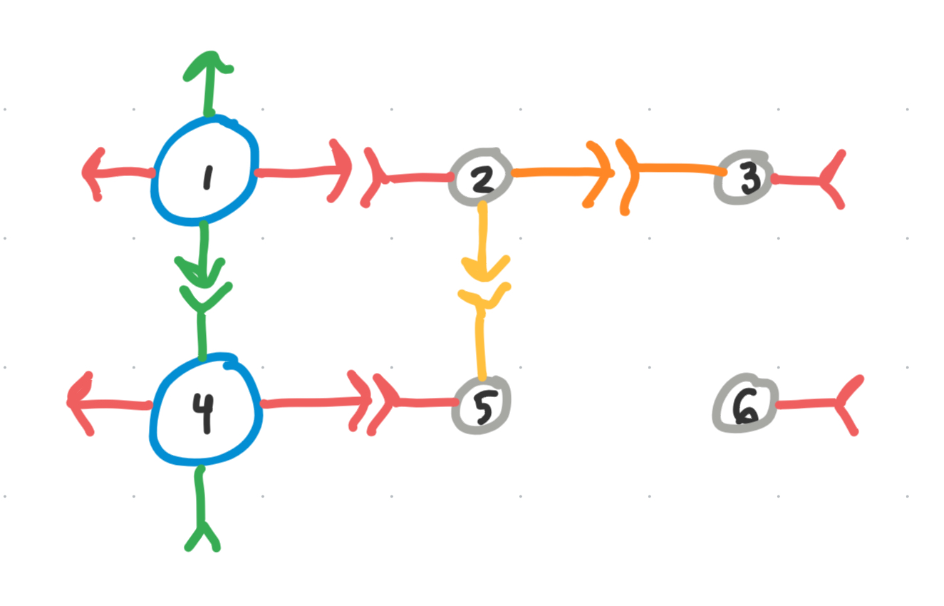
We can paint our third color in a similar fashion

Again breaking the equivalence class further:

\[\begin{align} [v_{2}] &= \{ v_{2}, v_{3}, v_{5}, v_{6} \} \\ \implies [v_{2}]^+ = &\{ v_{2}, v_{5}, v_{6} \}, \quad [v_{2}]^-= \{ v_{3} \} \end{align}\]

Note: We don’t technically know yet which sub-equivalence class $v_{5},v_{6}$ belong in, but we can assume they are in the parent one until forced out of it. For this reason we also hold off on mapping the orange onto them until we know for sure which sub-class they belong to.

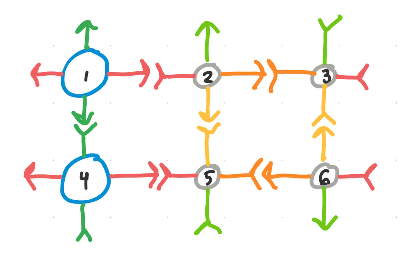
Our fourth color

Unfortunately, since $v_{2}$ does not have $90 ^{\circ}$ or $270 ^{\circ}$ self-symmetry, we must draw a fourth color from our palette to connect them.

Again, we have a breaking of the equivalence classes happening. But maybe, we can reuse the $[v_{2}]^-$ to avoid adding in a third subclass?

Hence, we get:

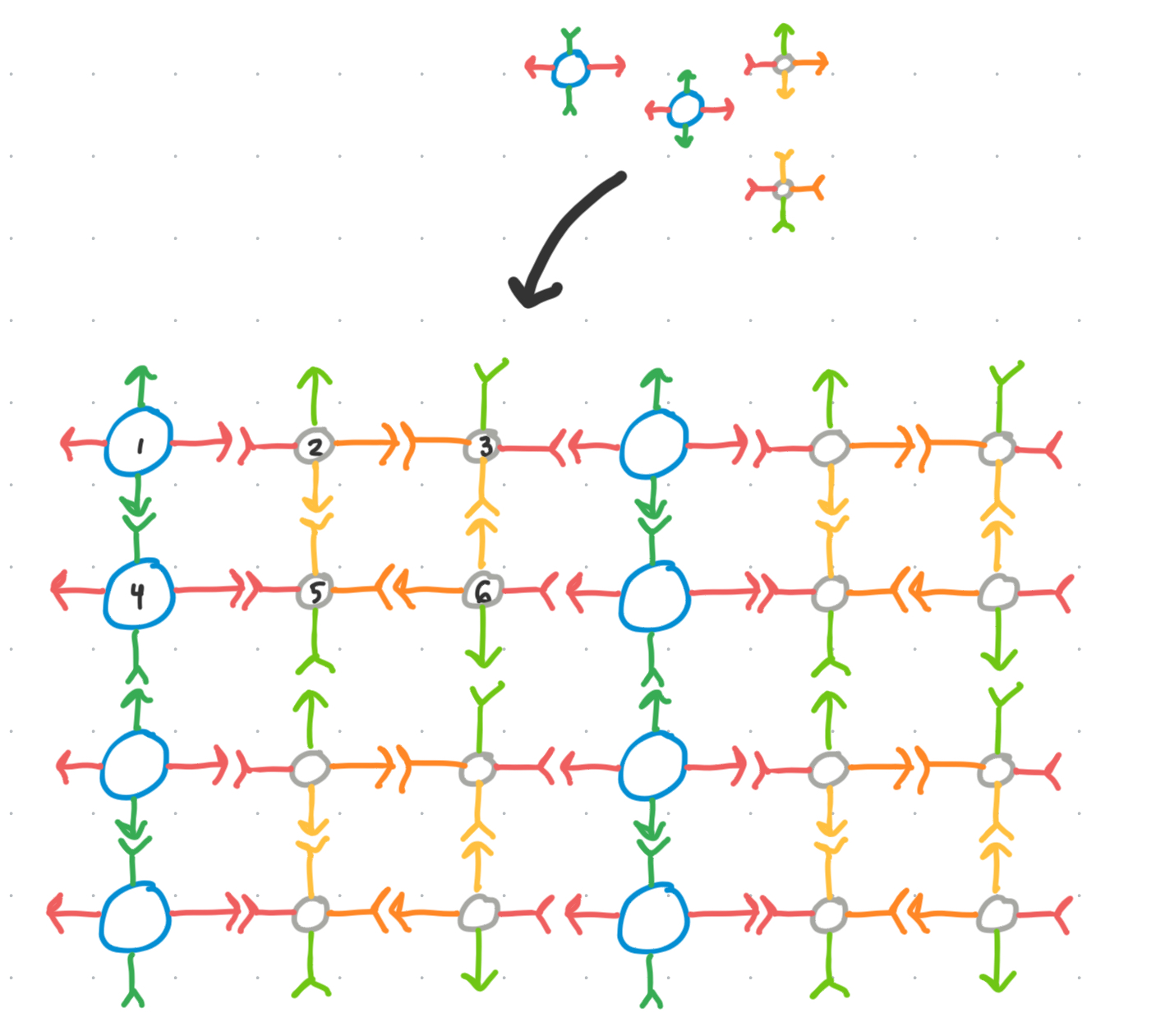
\[[v_{2}]^+ = \{ v_{2}, v_{6} \}, \quad [v_{2}]^-= \{ v_{3}, v_{5} \}\]

Since we have $v_{3}\in [v_{2}]^-$ as well with the orange color information, let’s reuse that for $v_{5}$ as well, alongside updating $v_{3}$ with the yellow information. ![[img13 1.jpeg|300]]

The last color

Now, we only need one more color to finish this!

And indeed, we end up with 4 unique origami:

\[\begin{align} [v_{1}]^+ &= \{ v_{1} \}\\ [v_{1}]^- &= \{ v_{2} \}\\ [v_{2}]^+ &= \{ v_{2}, v_{6} \}\\ [v_{2}]^- &= \{ v_{3}, v_{5} \} \end{align}\]

Which create a minimum set of building blocks which can self assemble into our desired infinite tiling structure!